How To Draw A Direction Field In Matplotlib

The aim of this mail is to guide the reader through plotting trajectories and direction fields for a system of equations in Python. This is useful when investigating the equilibria and stability of the arrangement, and to facilitate in agreement the general behavior of a organisation under study. I will use a organisation of predator-prey equations, that my almost devoted online readers are already familiar with from my previous posts on identifying equilibria and stability, and on nondimensionalization. Specifically, I'll exist using the Lotka-Volterra set of equations with Holling'due south Type Two functional response:

$\frac{\mathrm{d} x}{\mathrm{d} t}=bx\left ( 1-\frac{x}{K} \right )-\frac{axy}{1+ahx}$

$\frac{\mathrm{d} y}{\mathrm{d} t}=\frac{caxy}{1+ahx}-dy$

where:

10: prey abundance

y: predator abundance

b: casualty growth rate

d: predator death rate

c: charge per unit with which consumed prey is converted to predator

a: rate with which prey is killed past a predator per unit of time

G: prey conveying capacity given the prey'south environmental weather condition

h:handling fourth dimension

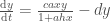
This system has 3 equilibria: when both species are dead (0,0), when predators are dead and the prey grows to its carrying capacity (Grand,0) and a not-trivial equilibrium where both species coexist and is mostly more interesting, given by:

$y^*=\frac{b}{a}(1+ahx^*)\left(1-\frac{x^*}{K} \right)$

$x^*=\frac{d}{a(c-dh)}$

The following code should produce both trajectories and direction fields for this system of ODEs (python virtuosos please alibi the extensive commenting, I try to annotate as much as possible for people new to python):

import numpy as np from matplotlib import pyplot every bit plt from scipy import integrate  # I'm using this style for a pretier plot, but it'south non actually necessary plt.style.use('ggplot')  """ This is to ignore RuntimeWarning: invalid value encountered in true_divide I know that when my populations are zero at that place's some sectionalization past aught and the resulting error terminates my function, which I want to avoid in this instance. """ np.seterr(divide='ignore', invalid='ignore')  # These are the parameter values we'll be using a = 0.005 b = 0.v c = 0.v d = 0.ane h = 0.one K = 2000  # Ascertain the arrangement of ODEs # P[0] is prey, P[ane] is predator def fish(P, t=0):     return ([b*P[0]*(1-P[0]/G) - (a*P[0]*P[1])/(1+a*h*P[0]),             c*(a*P[0]*P[ane])/(1+a*h*P[0]) - d*P[1] ])  # Define equilibrium betoken EQ = ([d/(a*(c-d*h)),b*(i+a*h*(d/(a*(c-d*h))))*(1-(d/(a*(c-d*h)))/Thousand)/a])  """ I need to define the possible values my initial points will take equally they relate to the equilibrium signal. In this example I chose to plot ten trajectories ranging from 0.1 to v """ values = np.linspace(0.1, five, 10) # I want each trajectory to have a different color vcolors = plt.cm.autumn_r(np.linspace(0.1, 1, len(values)))  # Open effigy f = plt.figure() """ I need to define a range of time over which to integrate the system of ODEs The values don't really thing in this case because our system doesn't have t on the correct manus side of dx/dt and dy/dt, but it is a necessary input for integrate.odeint. """ t = np.linspace(0, 150, 1000)  # Plot trajectories past looping through the possible values for five, col in zip(values, vcolors):     # Starting point of each trajectory     P0 = [E*5 for East in EQ]     # Integrate system of ODEs to get 10 and y values     P = integrate.odeint(fish, P0, t)     # Plot each trajectory     plt.plot( P[:,0], P[:,1],             # Unlike line width for different trajectories (optional)             lw=0.v*v,             # Different color for each trajectory             color=col,             # Assign starting point to trajectory label             label='P0=(%.f, %.f)' % ( P0[0], P0[ane]) ) """ To plot the direction fields we kickoff need to define a grid in order to compute the direction at each point """ # Get limits of trajectory plot ymax = plt.ylim(ymin=0)[one] xmax = plt.xlim(xmin=0)[one] # Define number of points nb_points = xx # Define ten and y ranges x = np.linspace(0, xmax, nb_points) y = np.linspace(0, ymax, nb_points) # Create meshgrid X1 , Y1 = np.meshgrid(10,y) # Calculate growth charge per unit at each grid point DX1, DY1 = fish([X1, Y1]) # Direction at each grid point is the hypotenuse of the casualty direction and the # predator direction. Thousand = (np.hypot(DX1, DY1)) # This is to avert whatsoever divisions when normalizing Yard[ M == 0] = i. # Normalize the length of each arrow (optional) DX1 /= Grand DY1 /= K  plt.title('Trajectories and direction fields') """ This is using the quiver office to plot the field of arrows using DX1 and DY1 for direction and M for speed """ Q = plt.quiver(X1, Y1, DX1, DY1, Grand, pivot='mid', cmap=plt.cm.plasma) plt.xlabel('Casualty affluence') plt.ylabel('Predator abundance') plt.fable(bbox_to_anchor=(1.05, 1.0)) plt.grid() plt.xlim(0, xmax) plt.ylim(0, ymax) plt.show()

This should produce the post-obit plot. All P0s are the initial conditions we divers.
trajectories

We can likewise see that this parameter combination produces limit cycles in our system. If we change the parameter values to:

a = 0.005 b = 0.5 c = 0.5 d = 0.1 h = 0.one K = 200

i.e. reduce the available resource to the prey, our trajectories await like this:

trajectories1

The equilibrium becomes stable, attracting the trajectories to it.

The same tin be seen if we increase the predator decease rate:

a = 0.005 b = 0.5 c = 0.5 d = one.5 h = 0.1 Yard = 2000

trajectories2

The implication of this observation is that an initially stable system, can go unstable given more resources for the casualty or less efficient predators. This has been referred to as the Paradox of Enrichment and other predator-prey models take tried to accost it (more on this in future posts).

P.S: I would also similar to link to this scipy tutorial, that I found very helpful and that contains more than plotting tips.